What You’ll Learn, and Why Most Explanations of RAG Miss the Point

You’ve almost certainly lived this scene. You ask an LLM (Claude, Gemini, ChatGPT) a precise question, hoping for an answer drawn from your own documents. The model replies with total confidence, in flawless English, citing facts that don’t exist. Not a subtle slip. A pure invention, delivered with the same poise as a verified truth.

This problem has a name: hallucination. And the architectural solution that has emerged to address it has another: RAG, short for Retrieval-Augmented Generation.

The concept is everywhere. Popular explainers sum it up in a single line: “you give documents to the model so it answers better.” That’s factually correct. It’s also spectacularly incomplete. Because RAG isn’t a button you switch on. It’s a pipeline: a chain of technical decisions in which every link (how you split your documents, how you turn them into vectors, how you store them, how you retrieve them, how you inject them into the prompt) determines the quality of the final result. And most of those decisions are invisible to the user.

If you’ve read my article on vectors, from Newton to the embeddings behind ChatGPT, you already have the core intuition: a piece of text can be projected into a mathematical space where geometric closeness mirrors closeness in meaning. RAG is the industrial application of that intuition. It’s the system that turns “these two texts are close in vector space” into “here is the answer to your question, with sources.”

This article covers the full mechanics of the RAG pipeline (from chunking to re-ranking) with data from the 2026 benchmarks, the concrete tools (NotebookLM, ChromaDB, LangChain), a taxonomy of approaches (closed, open, and hybrid RAG), and the traps beginners fall into every single time. All of it grounded in the FloTorch, HiCBench, and Firecrawl studies published over the past few weeks, and in the experience I’ve accumulated building my own AI stack.

If you take away just one thing from this introduction, let it be this: RAG is not a concept, it’s an engineering discipline. And like any discipline, it has its rules, its anti-patterns, and its shortcuts that cost you dearly.

Table of Contents

Toggle

RAG in One Picture: The Anatomy of a Pipeline

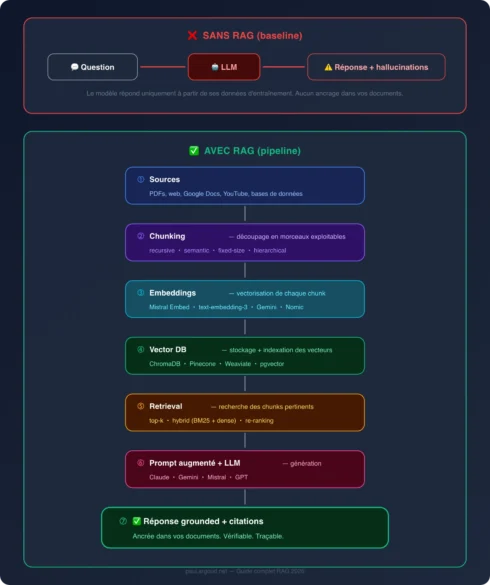
Before we get into the details, here is the complete flow of a RAG system. Each step is a technical decision that shapes every step after it.

The fundamental difference between the two diagrams comes down to a single word: grounding. Without RAG, the model draws on its training memory, which is frozen, incomplete, and sometimes wrong. With RAG, it draws on your documents, in real time, and can cite its sources.

Every stage of the pipeline deserves a closer look. Let’s start with the one that determines everything else.

Chunking: The Most Underrated Decision in the Pipeline

Chunking Strategies in 2026

An LLM doesn’t know how to search through a 200-page document, it knows how to read. Chunking solves this by cutting documents into pieces, indexing each piece on its own, and presenting the model with only the relevant ones. It’s the first move in the pipeline, and the one beginners botch most often.

Fixed-size. The simplest method: you cut every X tokens, full stop. It’s fast to implement and predictable. It’s also the method that produces the worst results in most cases, because it slices blindly through the middle of sentences, paragraphs, and ideas. A chunk that begins with “…of the European directive” and ends with “the report indicates that…” carries no usable meaning.

Recursive character splitting. The method that dominates the benchmarks. The principle: you try to cut by paragraph first, then by sentence, then by word, in a cascade. The result respects the natural boundaries of the text. The February 2026 FloTorch study (which compared seven chunking strategies under equal context budgets and standardized metrics) puts recursive splitting at 512 tokens at the top for both accuracy and retrieval F1. It’s LangChain’s default strategy, and it’s the one you should start with.

Semantic chunking. You use an embedding model to detect shifts in meaning and cut where semantic similarity drops. The idea is elegant. The reality is more nuanced: the FloTorch study shows that semantic chunking is often outperformed by plain recursive splitting, while costing significantly more (each cut requires an embedding call). That’s the paradox of 2026: the most sophisticated method isn’t always the best.

Hierarchical chunking. The most promising approach. You index the same document at several levels of granularity (paragraphs, sections, pages) and use parent-child relationships to navigate between levels. The HiCBench benchmark (September 2025, arXiv) shows gains of 18 to 25% in retrieval quality over flat approaches. The downside: implementation complexity is real, and the production tooling isn’t fully mature yet.

⚠️ Common mistake: purely fixed chunking with no overlap

This is beginner mistake number one. Fixed chunking at 512 tokens with no overlap produces cuts in the middle of sentences, lost context between adjacent chunks, and mediocre retrieval. The minimal fix: switch to recursive splitting with 10 to 20% overlap. The Firecrawl benchmarks (October 2025, NVIDIA/Chroma data) show that 15% overlap improves recall by 9% over zero overlap. It’s a free win: all you change is one parameter.

The Counterintuitive Insight of 2026

In January 2026, AI21 Labs published a study that challenges the very idea of a “good” chunk size. Their finding: the optimal chunk size depends on the query, not the document. A precise factual question (“What is the applicable VAT rate?”) benefits from small chunks (100–200 tokens). A synthesis question (“Summarize the tax implications of this contract”) benefits from large chunks (500–1,000 tokens). By indexing the same corpus at several sizes and aggregating the results with Reciprocal Rank Fusion, they obtain gains of 1 to 37% across benchmarks, without retraining a single model.

The practical takeaway: if your queries vary in nature, consider multi-scale indexing rather than a single chunk size. And if you’re just starting out, begin with 512-token recursive splitting and 15% overlap. That’s the baseline that works best across the widest range of cases.

⏩ Heads-up: even with excellent chunking, once you pass 10,000–50,000 chunks a new problem appears: retrieval starts returning semantically undifferentiated noise. This is semantic collapse, the subject of my next article.

Embeddings in 2026: Which Model to Choose (and, Above All, Not to Change)

Once your documents are chunked, you need to make them searchable. That’s the job of embeddings, the vectorization whose history and intuition I covered in an earlier article. Each chunk is turned into a list of numbers (768 to 3,072 dimensions) that encodes its meaning in a mathematical space. Two chunks on the same topic produce nearby vectors. That distance is measurable, and it’s what makes retrieval possible.

Embedding Models in 2026

The choice of embedding model matters less than the chunking strategy, but it’s not trivial:

The classic mistake: switching embedding models after you’ve already indexed your documents. Vectors from different models aren’t comparable, so changing means re-indexing the entire corpus. Choose well up front.

Vector DBs in 2026: ChromaDB, Pinecone, Weaviate, pgvector, Which One?

Before the comparison, one clarification is in order: a vector database is not a requirement for RAG. It’s the retrieval mechanism best suited to unstructured text corpora, but on structured data a SQL query does the same job. In a domain with a precise, stable vocabulary (legal, medical, regulatory), BM25 alone often beats vector search. And an open RAG system like Perplexity or Claude with web search touches no vector database at all: it fetches pages in real time. What defines RAG is the retrieve → inject → generate loop, not the technology that handles retrieval.

A classic relational database is optimized for exact queries (“give me the users named Dupont”). A vector database is optimized for similarity queries (“give me the 10 chunks closest to this question”). Nearest-neighbor search in a 1,024-dimensional space relies on specialized indexing algorithms (chiefly HNSW) that find approximate neighbors in near-constant time, even across millions of vectors.

The market is growing 22.3% per year (projected to reach $15.1 billion by 2034). Here are the main players:

ChromaDB: the entry point par excellence. Open source (Apache 2.0), one-line install (pip install chromadb), in-memory operation for prototyping, on-disk persistence for local production. The core was rewritten in Rust in 2025, with performance gains of up to 4x. As of February 2026, ChromaDB v1.5 natively supports vector search, full-text search (BM25 and SPLADE), regex search, metadata filtering, and multimodal embeddings (text + image via OpenCLIP). Its cloud service (Chroma Cloud) lets you go to production without managing infrastructure. It’s the tool I recommend for getting started: a working RAG pipeline in under 30 lines of Python.

The other players worth knowing:

Which one for which use case? Prototyping: local ChromaDB. Production with no infrastructure to manage: Pinecone or Chroma Cloud. Existing PostgreSQL stack: pgvector. Enterprise with hybrid search: Weaviate or ChromaDB.

Retrieval: top-k, Hybrid, Re-ranking, the Levers That Change Everything

Retrieval is the stage where the system looks for the chunks relevant to the question. The simplest method (top-k) turns the question into a vector and returns the k closest. It’s a good starting point, but two problems come up consistently in production.

Problem 1: semantic search misses lexical matches. If your question contains a technical identifier (“error ERR-4012”) or a proper noun, vector search may fail to find the chunk that holds that exact string, because embeddings capture meaning, not words. This is where hybrid search comes in.

Problem 2: top-k returns noise. Among the 10 or 20 closest chunks, some are relevant and others are merely close in vector space without being useful for the question. With no further filtering, that noise ends up in the LLM’s prompt and degrades the quality of the answer.

Hybrid Search: The Best of Both Worlds

Hybrid search combines vector search (dense retrieval, based on embeddings) with keyword search (sparse retrieval, typically BM25). BM25 is the classic search-engine algorithm: it finds documents that contain the same terms as the query, weighted by their frequency and their rarity.

By combining the two, meaning (vectors) and words (BM25), you get markedly more robust retrieval. ChromaDB has supported this approach natively since 2025, with first-class support for BM25 and SPLADE vectors alongside dense vectors.

Re-ranking: The Step Everyone Forgets

This is where the single most important insight of this article lives, and it’s the step most implementations neglect.

Re-ranking means taking the retrieval results (typically the 20 to 50 most relevant chunks) and re-ordering them with a more powerful model (a cross-encoder, or an LLM used as a judge) to keep only the best 3 to 5. Unlike vector search, which compares independently pre-computed vectors, the cross-encoder analyzes the pair (question, chunk) together, which lets it capture far finer relationships of relevance.

The February 2026 FloTorch study is categorical on this point: investing in re-ranking complexity yields measurable gains, whereas investing in chunking complexity often delivers diminishing returns. In other words, simple chunking with a good re-ranker beats sophisticated chunking with no re-ranking. That’s the exact opposite of what intuition suggests, and it’s why so many pipelines underperform.

Closed vs Open vs Hybrid RAG: The 2026 Taxonomy

The most defining distinction in 2026 isn’t technical, it’s architectural. It comes down to where the data the system uses to answer actually comes from.

Closed RAG: Everything Is Grounded in Your Sources

Closed RAG has access only to the documents you explicitly provide. No web access, no training memory as a source of truth: only your files. If the information isn’t in your sources, the system says so (or should).

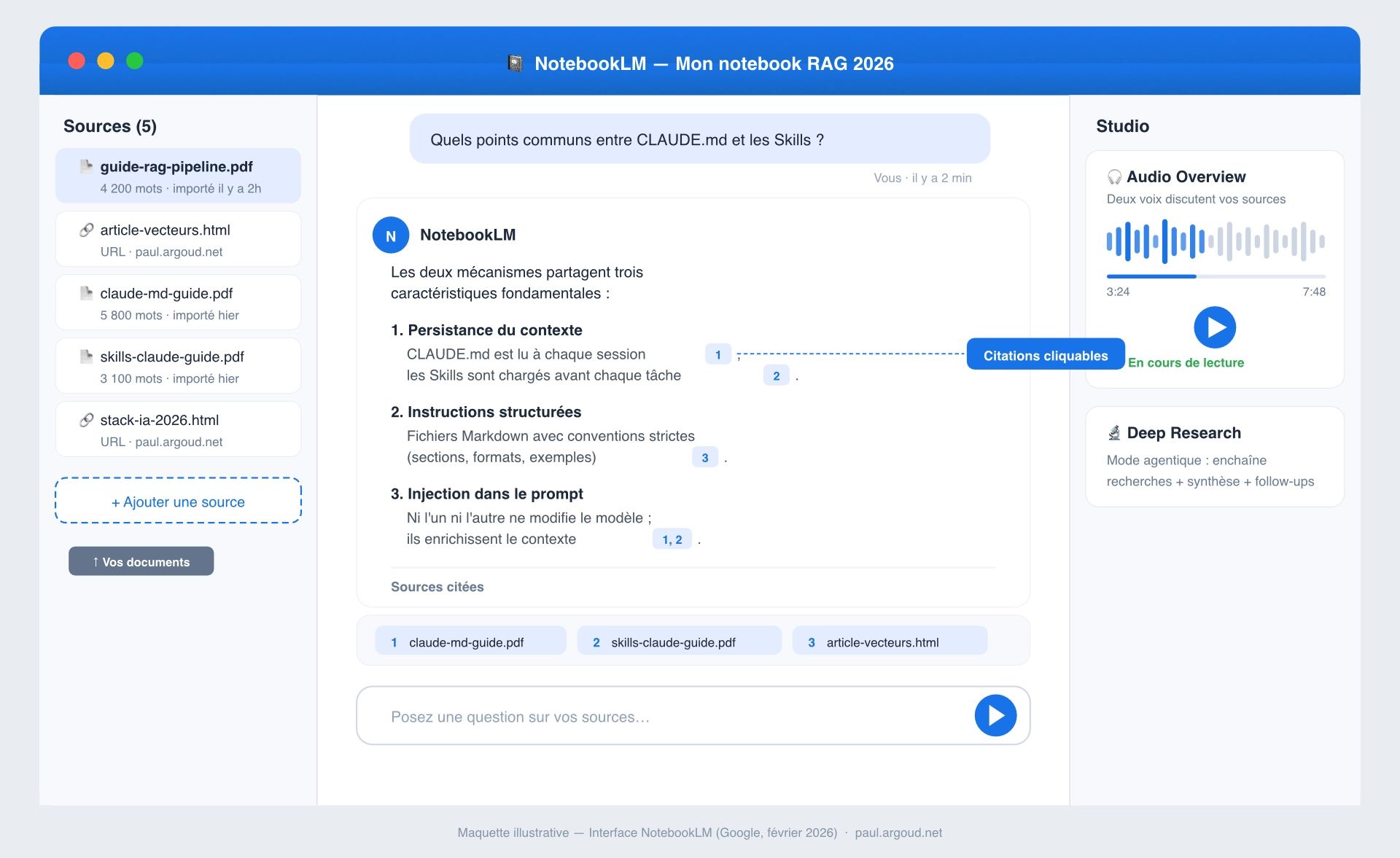
The archetype of closed RAG in 2026 is Google’s NotebookLM. You upload your documents (PDFs, Google Docs, web pages, YouTube videos, Google Sheets), and NotebookLM answers exclusively from those sources, with clickable citations that link back to the exact passage in the original document.

The advantages are considerable: zero risk of external hallucination (the model can’t invent what isn’t in your sources), controlled confidentiality (your data stays within the defined perimeter), and full traceability (every claim is sourced). The limits are the direct corollary: if your sources are incomplete, the system is “blind” to the topics they don’t cover.

Ideal use cases: academic research, contract analysis, literature reviews, meeting notes, training on an internal corpus.

Open RAG: Retrieval on the Web and Beyond

Open RAG goes out to fetch information from the web or from external databases, in addition to (or instead of) your own documents. Perplexity is the most visible example: every answer is built from web pages fetched in real time, with citations to the sources.

Claude with web search enabled, Gemini in standard mode, and ChatGPT with browsing all work on this principle. The power is obvious: access to current events, near-unlimited coverage, the ability to answer questions on topics you never documented.

The risks are proportional: noise in the results (the web is full of content of uneven quality), source bias (the model may favor popular sources over relevant ones), and hallucinations when retrieval brings back contradictory or off-topic information.

Hybrid RAG: The Best of Both Worlds (in Theory)

Hybrid RAG combines your private sources with external ones, under a hierarchy of trust. The system checks your documents first, then fills in from the web when needed.

NotebookLM took that step in November 2025 with the integration of Deep Research: the system can now search beyond your uploaded sources, but only if you explicitly allow it, and while keeping grounding on your documents as the priority. In December 2025, Google pushed the integration further by letting you attach a NotebookLM notebook directly inside a Gemini chat: this combines the rigor of closed RAG (your document base) with the power of open RAG (the web via Gemini), all in a single interface.

It’s this hybrid positioning that makes NotebookLM the best teaching tool for understanding RAG in 2026: it shows you, concretely, the difference between an answer grounded in your sources and an answer enriched by the web.

🔒 Confidentiality: what RAG exposes (and what it doesn’t)

Connecting your documents to an LLM through RAG does not make their contents accessible to the model’s other users. RAG injects your chunks into your prompt: that’s session context, not fine-tuning. The real question is whether the provider could use your data to train its future models. Paid and enterprise plans generally offer contractual commitments against this, but free plans come with vaguer clauses, and policies change over time. The only way to eliminate the risk entirely: host the model locally (Ollama, open-source LLMs). For sensitive documents: check the terms of service, favor paid plans, and consider local hosting if your confidentiality requirements demand it.

NotebookLM: RAG in Practice

Why Start with NotebookLM

If you’ve never worked with a RAG system, NotebookLM is where to start. Not because it’s the most powerful (a custom pipeline with ChromaDB will give you more control) but because it makes RAG visible. You see the sources cited, you see when the model can’t find the information, you see the difference between a grounded answer and an invented one.

Walkthrough: From Upload to Insight

Here’s a concrete use case. I’m going to use NotebookLM to analyze my own blog articles on AI, a corpus I know intimately, which lets me check the quality of the answers.

Step 1: Create a notebook and import your sources. Head to notebooklm.google.com. Create a new notebook. Upload your sources: PDFs, Google Docs, web pages (by URL), YouTube videos, or even Google Sheets. For my test: I import my five most recent technical articles by URL. NotebookLM supports up to 50 sources per notebook on the free tier, 300 on Pro (Google AI Pro, $19.99/month) and 600 on Ultra, a volume more than enough for most research projects.

Step 2: Explore with the chat. Once your sources are loaded, ask a cross-cutting question: something that requires connecting several documents. For example: “What do memory management in CLAUDE.md and the progressive loading of Skills have in common?” NotebookLM searches the relevant articles, synthesizes, and cites the exact passages. Every citation is clickable: you can verify that the model isn’t making anything up.

Step 3: Generate an Audio Overview (the podcast). This is NotebookLM’s signature feature. The tool generates a 10-to-15-minute “podcast” in which two synthetic voices discuss your sources with an unsettling naturalness. This is no gimmick: it’s a remarkably effective learning tool. Hearing your own documents summarized and discussed by an AI surfaces connections you hadn’t seen on the page. The interactive mode, available in the Deep Dive format, even lets you ask the podcast questions while it plays.

Step 4: Turn on Deep Research (hybrid RAG). NotebookLM has included Deep Research since November 2025. Since January 2026, it runs in fully agentic mode: the system chains together several autonomous searches beyond your sources, synthesizes the results, and proposes follow-ups. Launch a deep search on a topic related to your documents: NotebookLM will go out to the web, bring back a structured report with dozens of sources, and let you import them into your notebook to enrich your base.

Step 5: Connect to Gemini. Since January 2026, you can attach your notebook directly inside a Gemini chat through the attachment menu. Gemini then has access to your document base while keeping its conversational abilities, Canvas, and Deep Research. It’s the most powerful combination in the Google ecosystem in 2026: the rigor of closed RAG plus the flexibility of open RAG.

NotebookLM’s teaching value goes beyond its practical usefulness. Using it, you watch the fundamental phenomena of RAG play out in real terms: how retrieval selects passages, how the system handles contradictions between sources, and how the quality of the sources determines the quality of the answers.

The Other Managed Services: RAG Without a Pipeline

NotebookLM isn’t the only one. Several services offer turnkey RAG: Perplexity (open RAG geared toward web search, every answer sourced), Anthropic’s Claude with Projects (upload documents and Claude uses them as context: lightweight closed RAG with Claude’s reasoning quality), Gemini with Google Drive (direct access to your files, enriched by the NotebookLM integration), and the enterprise solutions (Pinecone, Weaviate Cloud, Chroma Cloud: managed vector databases with built-in ingestion pipelines).

The rule of thumb: if you’re exploring, start with NotebookLM. If you need control, build with ChromaDB. If you need to scale without ops, move to a managed cloud.

ChromaDB: Building Your Own RAG Pipeline

NotebookLM is a closed tool: you control neither the chunking, nor the embeddings, nor the retrieval, nor the prompt. For a chatbot on your product documentation, a domain assistant, or an extraction pipeline, you need to control every parameter. That’s where ChromaDB comes in, and more broadly frameworks like LangChain and LlamaIndex.

A Minimal RAG Pipeline in Python

Here is a working RAG pipeline in Python with ChromaDB. This isn’t a toy: it’s the structure you can extend for a real use case.

import chromadb
from chromadb.utils import embedding_functions

# 1. Initialize ChromaDB (in-memory for prototyping)
client = chromadb.Client()

# Or with on-disk persistence:
# client = chromadb.PersistentClient(path="./chroma_db")

# 2. Choose an embedding model
# Default: all-MiniLM-L6-v2 (free, local)
# For production, consider OpenAI or Mistral Embed
embedding_fn = embedding_functions.DefaultEmbeddingFunction()

# 3. Create a collection (= an index)
collection = client.create_collection(
    name="my_documents",
    embedding_function=embedding_fn
)

# 4. Add chunks with metadata
# In production, these chunks come from your chunking pipeline
collection.add(
    documents=[
        "RAG grounds an LLM's answers in the documents you provide.",
        "Recursive chunking respects the natural boundaries of the text.",
        "ChromaDB supports vector search and full-text search.",
        "Re-ranking with a cross-encoder improves retrieval precision.",
    ],
    metadatas=[
        {"source": "intro.pdf", "section": "definition"},
        {"source": "chunking.pdf", "section": "strategies"},
        {"source": "chromadb.pdf", "section": "features"},
        {"source": "retrieval.pdf", "section": "optimization"},
    ],
    ids=["chunk_1", "chunk_2", "chunk_3", "chunk_4"]
)

# 5. Retrieve the chunks relevant to a question
results = collection.query(
    query_texts=["How can I improve retrieval quality?"],
    n_results=3  # top-k = 3
)

# 6. The results contain the chunks, distances, and metadata
for doc, metadata, distance in zip(
    results["documents"][0],
    results["metadatas"][0],
    results["distances"][0]
):
    print(f"[{distance:.4f}] {metadata['source']} → {doc[:80]}...")
Code language: Python (python)

Expected output (example):

[0.3412] article_rag.pdf → Re-ranking is the most underrated lever in the RAG pipeline. FloTorch show...
[0.4298] article_rag.pdf → Hybrid search combines vector (semantic) similarity with BM25...
[0.5107] guide_chunking.md → Fixed-size chunking with no overlap produces chunks without full context...
Code language: CSS (css)

What happens under the hood: ChromaDB turns your question into a vector (using the same embedding model that indexed the chunks), computes the cosine distance against every stored vector, and returns the n_results closest. The metadata (source, section) lets you filter the results: for example, searching only within a specific document or a given section.

From Prototype to Production

The code above is a starting point. For a production pipeline, you’ll add:

A real chunking pipeline. LangChain provides ready-made chunkers (RecursiveCharacterTextSplitter, SemanticChunker) that handle overlap, custom separators, and respect for sentence boundaries.

A production embedding model. Replace the default model with Mistral Embed (for a French-language corpus), OpenAI text-embedding-3-large (general quality), or Nomic Embed (good value).

Hybrid search. ChromaDB supports BM25 natively: turn it on to combine semantic search with keyword search.

Re-ranking. Add a cross-encoder (such as Sentence Transformers’ cross-encoder/ms-marco-MiniLM-L-12-v2) or use an LLM as a judge to re-order the retrieval results before injecting them into the prompt.

Monitoring. Track your retrieval metrics (recall, precision, MRR, nDCG) over time. Frameworks like RAGAS provide standardized evaluation tools for RAG pipelines.

📊 How do you evaluate your RAG? Three essential metrics

You can’t improve what you don’t measure. Three metrics cover the essentials:

Retrieval Recall@5: of your top 5 returned chunks, how many are actually relevant? If you’re below 80%, your chunking or your embedding model is the problem.

Faithfulness: is the LLM’s answer faithful to the injected chunks, or does it hallucinate beyond them? A low score signals a poorly designed prompt or chunks too short to supply enough context.

Answer Relevance: does the final answer actually address the question asked? A low score combined with good recall points to a problem on the generation side, not the retrieval side.

Frameworks like RAGAS and Patronus AI automate these measurements. Build them in from the start, not after your first production bug.

Pitfalls, Troubleshooting, and Best Practices

Five Recurring Symptoms and Their Causes

“The answers are off-topic or incomplete.” Almost always the cause: chunking. Fixed-size chunking with no overlap produces chunks with no complete meaning. Fix: recursive splitting with 10–20% overlap. If the problem persists, try semantic chunking or increase to 400–600 tokens.

“Lots of noise in the results.” Retrieval brings back chunks that are “close” but not relevant. Levers: metadata filtering (filter by date, author, section before the vector search) and hybrid BM25 + dense search.

“The model hallucinates despite good sources.” The relevant chunks are drowned among irrelevant ones in the prompt. Fix: re-ranking with a cross-encoder or LLM-as-judge, top-20 → top-5.

“API costs are exploding.” Inefficient retrieval = too many chunks sent to the LLM. Fix: better chunking + pre-LLM re-ranking to filter before sending.

“Long context gets lost.” The “lost in the middle” phenomenon, documented by Stanford/Berkeley back in 2023: LLMs handle information placed at the beginning and end of a prompt better, and “forget” what sits in the middle. Fix: limit to 3–5 injected chunks, place the most relevant ones at the start and end of the prompt, and use 400–600 token chunks with 100–150 token overlap.

Summary Table

Pre-Production Validation Checklist

Before you start:

• [ ] You’ve identified the type of RAG suited to your case (closed, open, hybrid)
• [ ] You have a test corpus with questions and expected answers
• [ ] You’ve chosen an embedding model and don’t plan to switch midstream

While building:

• [ ] Your chunking respects sentence boundaries (no cuts mid-sentence)
• [ ] You have 10 to 20% overlap between chunks
• [ ] Your chunks carry metadata (source, date, section)
• [ ] You test multiple chunk sizes if your queries vary
• [ ] Your retrieval combines vector and BM25 (hybrid search)
• [ ] You have a re-ranking step before injection into the prompt

After deployment:

• [ ] You measure the recall and precision of your retrieval
• [ ] You track the hallucination rate on a sample of questions
• [ ] You have a re-indexing process for when your sources change
• [ ] You measure cost per query and identify possible optimizations

The Last Word

RAG is now the essential building block of productive AI. It’s what turns an LLM (brilliant but amnesiac) into an assistant anchored in your data, able to cite its sources and acknowledge the limits of what it knows. Without RAG, an LLM is a charismatic speaker improvising. With RAG, it’s an analyst working from files.

But as you scale (thousands of documents, ever-growing corpora, giant context windows trying to swallow everything) a question arises: what if RAG, by recycling more and more similar contexts, were preparing its own obsolescence? When your corpus holds thousands of semantically close chunks, retrieval starts returning undifferentiated noise: a phenomenon some researchers call semantic collapse.

That’s exactly the subject of my next article. In the meantime, here’s a concrete exercise: upload your five most recent documents into NotebookLM. Ask a cross-cutting question that requires connecting several of them. Watch what the system retrieves, what it cites, and what it misses. Then launch an Audio Overview and listen to your own documents narrated by two synthetic voices. It’s uncanny. It’s effective. And it’s the best way to understand viscerally what RAG does, and what it doesn’t do yet.